ITK-SNAP Segmentation of Stroke-related Lesions
Introduction
What is a Lesion Mask?
It can be valuable to mask lesions. Lesion masking involves creating a layer that covers the lesion (and only the lesion). In the picture below, you see an axial slice through a brain with a large lesion. On the right, we have covered the lesion with a red mask (translucent so you can see what is underneath). Most often we mask lesions manually. Lesion masks are sometimes referred to as lesion maps or as segmentations.
Manual masking of lesions can take hours or days because we need to outline the lesion carefully on each slice of the image. But this mask took only a few minutes to generate in ITKSNAP, and although it will need to be edited, it is a good start.
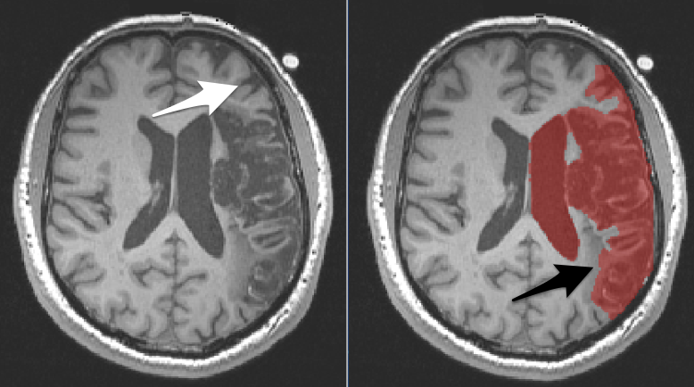
To determine whether an area should be included in the lesion mask, compare the tissue on the damaged side to the normal tissue in the other hemisphere.
- There are two arrows on the above images:
- Left The white arrow points to a region that is incorrectly covered by the mask. This is a sulcus and the normal looking grey matter that wraps that sulcus. You can see similar structures in the other hemisphere.
- Right The black arrow points to a region that should be covered by the mask, but isn’t. The discolored region is not comparable to anything in the other hemisphere. It is dark like grey matter, but does not wrap a sulcus and is in an area that should be white matter.
- The ventricle is also covered by the mask, but really we want only the enlarged portion of the ventricle to be covered by the mask…not the entire ventricle. We did this on purpose and will fix it later.
ITK-SNAP’s semi-automated and manual techniques help make lesion masking faster and more reproducible than the traditional fully manual approach. Here we review a semi-automated approach to segmentation of stroke-related lesions. For more tips on working with large lesions, see the Stroke Lesions page.
Why Create a Lesion Mask?
Here are some reasons to mask a lesion:
- You want to measure the volume of the lesion (so you measure the volume of the mask).
- You want to normalize the brain into standard space, so you mask the lesion to indicate that the tissue under the mask should not be considered (because the tissue under the mask is abnormal). This is important for many normalization routines.
- You want to run statistical analyses on lots of lesions to determine how the lesion location and size might affect behavioral measures. Explore Voxel Based Morphometry (VBM) and Voxel Lesion Symptom Mapping (VLSM) to learn more.
Goals
Learn to use ITK-SNAP segmentation software to create an initial lesion mask. In this pipeline we fill the lesion in the left hemisphere without worrying about leaking into ventricles or outside the brain, because we will fix those problems later using FSL.
Data
A dataset, T1w_defaced.nii.gz was kindly provided by A. Kielar. It consists of one native space defaced T1 weighted anatomical image of a patient with a large stroke-related lesion. The data has isotropic voxels which makes it optimal for semi-automatic segmentation in ITK-SNAP. Anatomical MRI data like this must have the face removed in order to deidentify it before posting it publicly. More information about how the data were collected is available here:
Kielar, A., Deschamps, T., Jokel, R., and Meltzer, J. A. (2016). Functional reorganization of language networks for semantics and syntax in chronic stroke: Evidence from MEG. Human Brain Mapping, 37(8), 2869-2893. doi: 10.1002/hbm.23212 PMID:27091757
Setup
First you will need to install ITKSNAP and open T1w_defaced.nii.gz. See Load and View Images.
Select a Region of Interest for Automatic Segmentation
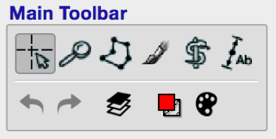
- Make sure the Crosshair mode is selected (leftmost icon on Main Toolbar). When you move the 3D crosshairs in one view, they move in the other views as well.
- Position the 3D crosshairs in the center of the lesion (look at all three views).
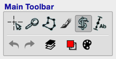
- In the Main Toolbar, select the Active Contour Tool (the snake and staff).
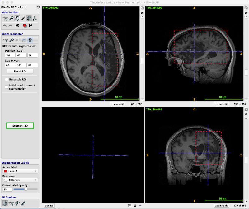
- Using the left mouse button, drag the corners of the active contour selection box, so that the box encompasses the lesion and enlarged ventricles as shown below.
- Use the scroll bars on the right of each image to ensure you have tightly enclosed the entire lesion (including damaged tissue that may surround the CSF). We will worry about excluding the normal extent of the ventricles later.
- Press Segment 3D (green box, middle left of figure below) to crop the image to the box.
- In the Segment 3D panel, ensure that Current Stage = Step 1/3 Presegmentation Mode; Actions = Thresholding (blue box, upper right in the figure below).
- You have now produced the speed image. This is a simplified blue and white segmentation.
- Press the little icon in the right top corner of any of the three slice views (3 tiny green boxes in figure below).
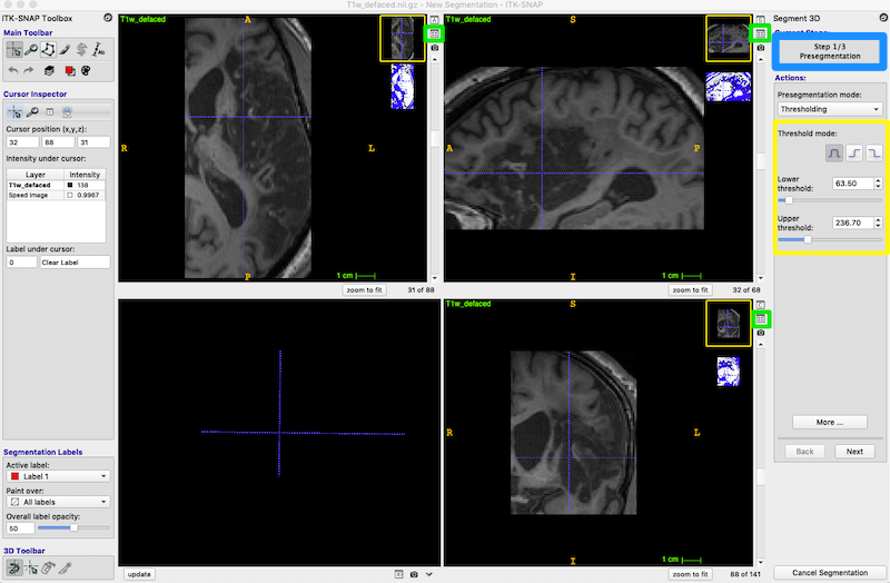
- This icon toggles between the thumbnail view of the speed image (shown above) and the side_by_side view (shown below).
- Side-by-side view is easier to use in the following steps.
- If you want the images to fill the available space, try the zoom to fit button (orange box, figure below)
Segment the Lesion
Thresholding to Isolate the Lesion
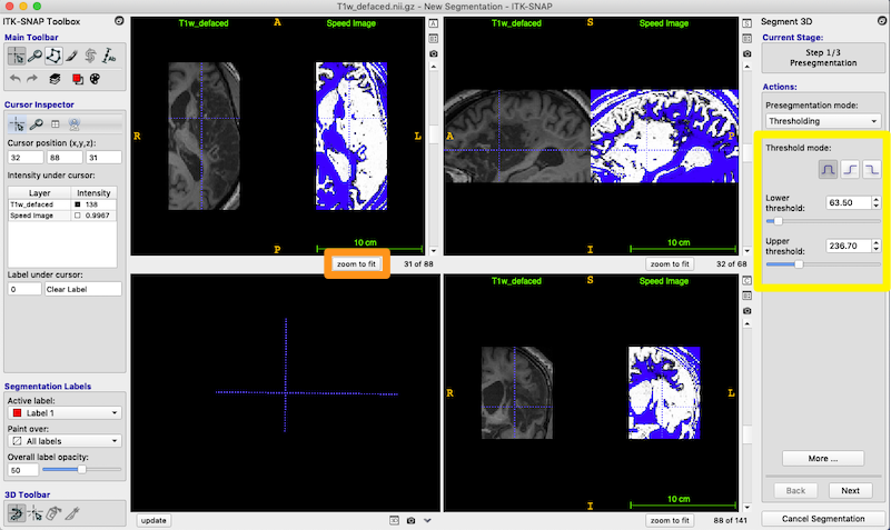
- Your speed image probably does not look like the one pictured, because the default thresholds are wrong. Now that you are viewing the T1 and speed image side-by-side, you should adjust the thresholds (yellow box on the right).
- Set the lower and uppper thresholds as shown. Your goal is the make the lesioned tissue as white as possible in the speed image, but keep the non-lesioned tissue blue. You should play with the settings.
- white=lesion
- blue=non-lesion
Note
The Threshold mode we use is the first of the 3 icons (yellow box, figure above): the complete waveform represents having both an upper and lower threshold. Choose each of the other icons to understand how they control thresholding.
- Press Next on the bottom right of the Segment 3D panel to continue. (You can go back without losing anything).
- You are now on Step 2/3: Initialization mode
An Alternative: Clustering to Isolate the Lesion
Thresholding works well when you have a single high quality image, as provided for this tutorial. However, if you have multimodal data (e.g., T1w, T2w, DWI), then you may benefit from using clustering instead of thresholding. The clustering approach can use converging evidence from all of the images to identify the lesion. Clustering may also do a better job than thresholding of identifying regions that are heterogenous and thus not well defined by thresholding.
If you have multiple images, they must have isotropic voxels and be coregistered. See these useful tools if you don’t have a preferred way to achieve isotropic voxels and coregistration. The video multimodal segmentation in ITK-SNAP provides a good introduction to the clustering approach.
- To use clustering instead of thresholding, choose Clustering from the Presegmentation mode dropdown box (figure below).
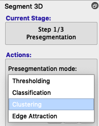
- Instead of Upper and Lower thresholds, you will see Number of clusters and Foreground cluster. By default, the speed image displays the first cluster in the foreground, but you can click the selector next to Foreground cluster to see more identified clusters. You can also increase or decrease the number of clusters to discover whether the tissue you want is identified reasonably well. Usually 3-5 clusters will do the job.
You could use clustering even with a single image like this one. Clustering may do a better job of identifying damaged tissue. Keep in mind that you are not limited to doing a single segmentation. You could create multiple segmentations and then combine them.
Set Segmentation Labels
- Segmentation labels are optional for this tutorial because you will only have one segmentation mask open at a time. Nevertheless, it is a good idea to learn how to label different segmentations, so let’s do it.
- Follow the instructions in the labels section to change Label 1 to Lesion
- Set the Active label = Lesion once you have changed the name.
- For the active label, set Overall label opacity = 50. This insures 50% opacity, so you can see the anatomical image under the label. You will need to watch how much of the region is filled by the lesion label, so you know when to stop the process.
Place Bubbles
Okay, that was a long detour from the task at hand, but you have learned about clustering and labeling. Now, as you may recall, we are on Step 2/3: Initialization mode. We are going to use thresholding for the remainder of the lesson.
- In this step, you place bubbles to initialize the active contour.
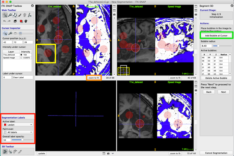
- First, check that the Segmentation Labels are set correctly (red box, figure below). The bubbles will be red and 50% opacity.
- Use the 3D crosshair cursor to select a location in the middle of the lesion.
- Under Actions, press Add Bubble at Cursor to insert an initialization bubble (green box, upper right of figure below).
- Place initiation bubbles on various slices to cover examples of both damaged tissue and the heterogeneous CSF-filled portion of the lesion. The figure below shows numerous bubbles on the image and in the Active bubbles table on right of the figure.
- In the figure below, I have put a yellow box around one of the bubbles. This bubble was not placed very carefully, and you can see that it overlaps good tissue next to the ventricle. Don’t worry! This is fine. When we get to the next step the bubbles will morph to fill the lesioned tissue and shrink away from the healthy tissue.
- Scroll through each of the three orthogonal views to ensure you have a good selection of bubbles. You can delete bubbles or change their sizes from the Active bubbles table on the right.
Note
As you scroll through the slices, the bubbles appear to change size. This is because they are spheres, so they appear smaller as you move away from their centers.
- Press Next in the Segment 3D panel on the right to continue. You can always go back without losing your work.
- You are now on Step 3/3 Evolution.
Run Active Contour Segmentation
- In Step 3/3 Evolution, you grow the bubbles to fill the lesion.
- Press Set Parameters (red box on right of figure below) to bring up the Active Contour Evolution Parameters window shown below.
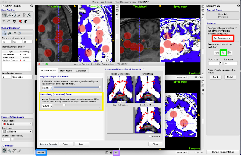
- Set Smoothing (curvature) force to 0.8 (yellow box, figure above) and press Close on the Active Contour Evolution Parameters window. This will prevent the bubbles from growing long spindly fingers, which is good because we want to discourage the bubbles from growing into every sulcus they encounter.
- To see your bubbles in 3D, press the update button under the 3D panel (blue box, lower left of figure above).
- Alternatively, select the down arrow in the bottom center of the figure below (tiny purple box, figure above). You can choose Continuous Update to watch the 3D shape emerge as the contour evolves.
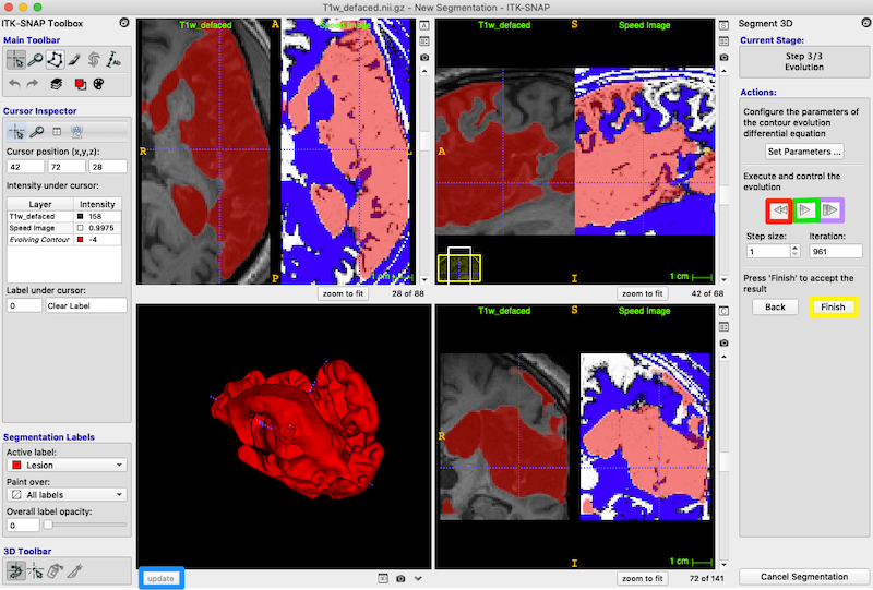
- Under Actions, press the play button (green box on middle right) to start evolution. It changes into a pause button. After about 950 iterations, press the pause button to stop the evolution.
- You can evolve the contour one iteration at a time with the button to the right of the play/pause button (purple box, middle right of figure below).
- If you are not using Continuous Update, then as the contour evolves, you can pause the evolution and update the 3D view. Again press the update button under the 3D panel to see the 3D shape.
- If you are not satisfied with the segmentation, you can return to the original unevolved bubbles with the button on the left of the play/pause button (red box on middle right of the figure below).
- Exit semi-automatic segmentation mode: On the right, under Actions, press the Finish button (yellow box, on the right in the figure below). You can always click update to get the latest 3D rendering of the lesion structure.
Note
In the 3D panel, use the right-mouse to change zoom level on the 3D volume, and the left-mouse to rotate the 3D volume. You can also move the 3D volume by moving the sliders on the other three panels.
Save Workspace
Before editing the segmentation, let’s save our work as a workspace in ITK-SNAP. This will include saving the segmentation mask we just created.
- From the ITK-SNAP menu, select Workspace → Save Workspace As
- ITK-SNAP complains that the segmentation image does not have a filename.
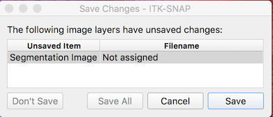
- Press Save and choose a name and location for your segmentation file (e.g., sub-001_lesion_mask.nii.gz).
- You will now be asked to save the workspace. Choose a workspace name and location as well (e.g., sub-001.itksnap in the same directory as the segmentation).
- Now you can easily load the anatomical image and any segmentations by choosing the workspace from the menu.
Editing the Segmentation
Now we want to evaluate and edit our work. We can do some of this with ITK-SNAP, but FSL also offers some useful tools. The lesion may have leaked into neighboring ventricles or even outside of the brain. Both 2D and 3D editing tools are available in ITK-SNAP. See 2D segmentation for more information about using these editing tools.
You now have experience with semi-automated and manual segmentation tools in ITK-SNAP. Next, I introduce you to additional tools that can be used to clean up the mask you created. Most of these tools depend on FSL and the UNIX command line. So this is a much deeper dive into the NIFTI image format and associated thorny problems. If you don’t have any experience with the command line, this might be a good time to take a break. If you are comfortable at the UNIX command line and already have FSL installed, then you will want to download some additional scripts as described below, and put them in your path.
Continue to the section Create a Brain Mask.