Choropleth Visualization
Introduction
Choropleths are simple maps that display regional changes as color (e.g., a US map showing states that lean Democrat vs Republican). Here is an example of a brain choropleth.
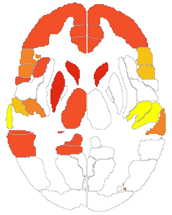
We demonstrated that this simple approach to visualization works well for brains, and, in fact, facilitates analysis:
Obviously brain choropleths are most valueable if you can choose the slice to view and display information about the regions in each slice. The original dynamic Weave visualizations allowed slice stacking. However, you will need to enable Adobe Flash to view the Weave visualizations, and Weave is no longer available. For this reason, we needed a new implementation. See Devin Bayly’s Neuro-choropleths Tool. This work was supported by the University of Arizona HPC center. It uses Javascript to display GeoJSON slices and regional information. Devin’s implementation of brain choropleths is fast and easy to use. You can make notes, compare different views and export your session to load up later.
roixtractor
Even without the brain visualizations, extraction of regional descriptive statistics provides a lot of power for analysis. You can extract such data by region using a Docker container that includes FSL 5.X and the scripts and atlases for extraction. See the roixtractor app provided as part of the scif_fsl tools. The scif_fsl Readme provides more detail. You will need to install Docker to run the tools. The git repository for roixtractor includes all the atlas ROIS, if you are curious.
Note
Docker can be run on some Windows machines, but it requires at least the professional version of Windows 10. You may have trouble with Docker on older operating systems.
Once Docker is installed, you can obtain an up-to-date copy of the scif_fsl Docker container by pulling it from dockerhub:
docker pull diannepat/scif_fsl
After downloading the Docker container to your local machine, I suggest getting a copy of the wrapper script sfw.sh which facilitates querying and calling the tools in the Docker container. Put this script somewhere in your path. You can begin by running the script with no arguments:
sfw.sh
Running sfw.sh will provide a list of apps in the container and relevant help for using them. roixtractor is one app in the container and is useful for extracting descriptive statistics for each region in a standard MNI 2mm image. You can try the test statistical image run-01_IC-06_Russian_Unlearnable.nii.
To run roixtractor you must pass it: 1) A statistical image in 2mm MNI standard space 2) A statistical threshold (output regions must be equal to or greater than this value) 3) An available atlas: HO-CB or HCP-MMP1:
- HO-CB: The Harvard-Oxford cortical and subcortical atlases combined with a cerebellar atlas.
- HCP-MMP1: Although it is possible to output these values in HCP-MMP1 space, it is probably not a good idea to use the HCP-MMP1 atlas in volumetric space. It is not likely to be terribly accurate).
Here is an example run:
sfw.sh xtract run-01_IC-06_Russian_Unlearnable.nii 1.5 HO-CB
This uses the keyword xtract to call the correct app. In this example we pass in a NIfTI stats image in 2mm MNI space: run-01_IC-06_Russian_Unlearnable.nii. The threshold value is 1.5, and the atlas is HO-CB.
Given the above command, roixtractor will generate a NIfTI file and two CSVs:
- NIfTI file with the mean value displayed in each region that meets criterion. This can be viewed in any NIfTI viewer.
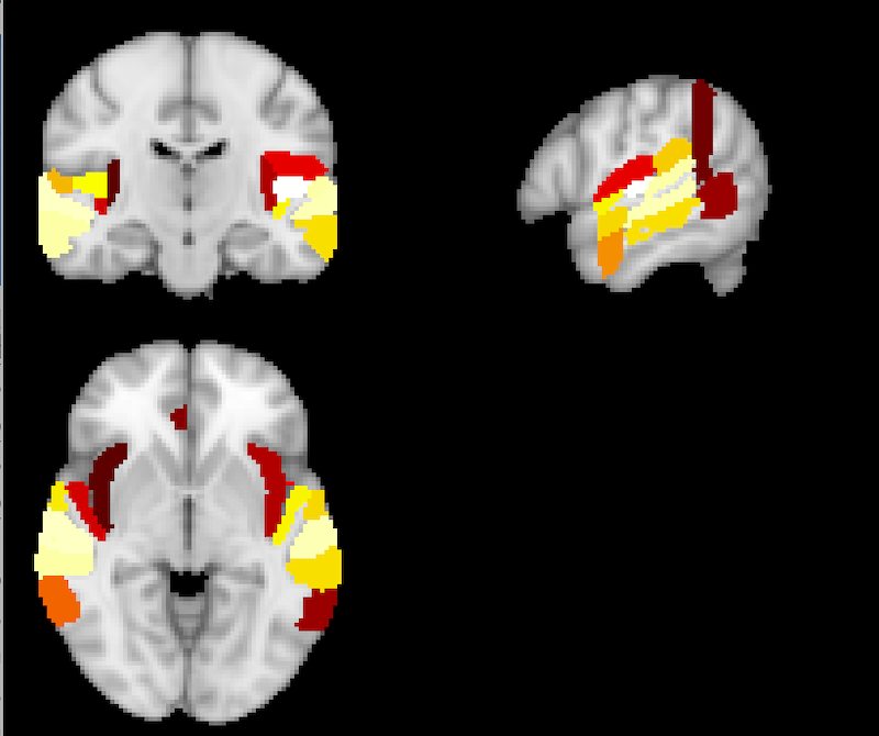
FSLeyes displays the regions in the hybrid HO-CB atlas that meet the threshold criterion. The image, HO-CB_run-01_IC-06_Russian_Unlearnable_1.5.nii.gz, generated by running the above command, is named with the atlas name: HO-CB prepended and the threshold value 1.5 appended.
- The first CSV (e.g.,
HO-CB_run-01_IC-06_Russian_Unlearnable_1.3.csv), like the NIfTI file, contains only the regions that meet your criterion threshold. This CSV will contain the following fields: Region, Mean, Max, SD, LR, Lobe, CogX, CogY, CogZ, RegionLongName, RegionVol_MM3, Image. - For example: BA44_R,1.664311,2.824052,0.597232,R,Fr,19,71,44, Inferior_Frontal_Gyrus_pars_opercularis_R,5240,run-01_IC-06_Russian_Unlearnable_1.5
- Region: the short region name
- Mean, Max and SD are descriptive statistics for each region.
- LR: identifies the region as left or right (redundant, but useful for sorting)
- Lobe: The lobe in which that region is found
- CogX, CogY and CogZ: are the x,y,z center of gravity voxel coordinates for each region
- RegionLongName: A more detailed name for the region if available
- RegionVol_MM3: The volume of the region in cubic mm
- Image: The name of the image you passed to the program: the name of the atlas you used is prepended and the threshold you used is appended to the name. Because image is the last field in the spreadsheet, you can easily use Excel to split the data on underscores. This splitting is useful if you want to concatenate several CSVs from different runs of the xtractor.
- The second CSV file (e.g.,
HO-CB_run-01_IC-06_Russian_Unlearnable_1.3_LI.csv) contains laterality information based on Wegrzyn, M., Mertens, M., Bien, C. G., Woermann, F. G., & Labudda, K. (2019). Quantifying the Confidence in fMRI-Based Language Lateralisation Through Laterality Index Deconstruction. Frontiers in Neurology, 10, 1069–15. http://doi.org/10.3389/fneur.2019.00655
The number of Suprathreshold voxels in each region is reported for left and right homologs. Strength=L+R; Laterality=L-R; LI=Laterality/Strength.
Resources
- Patterson, D. K., Hicks, T., Dufilie, A. S., Grinstein, G., & Plante, E. (2015). Dynamic Data Visualization with Weave and Brain Choropleths. PLoS ONE, 10(9), e0139453–17. http://doi.org/10.1371/journal.pone.0139453: This is the original choropleth paper.
- Neuro-choropleths Iodide Notebook: Devin Bayly, with support from the University of Arizona HPC center, is working on this implementation of a choropleth viewer.
- Sample 3D stats image: run-01_IC-06_Russian_Unlearnable.nii.
- Geo_NIFTI.zip: The regions in NIfTI format for our HO-CB hybrid atlas. This includes ROIS.zip which is individual binary masks for each region and HO-CB_all.nii.gz which combines all the label regions and can be downloaded and used for display of the regions in the hybrid atlas.
- HO-CB GeoJSON files. Only for the curious
- HCP-MMP1 GeoJSON files. Only for the curious
- CreateGeoJSON.zip: Bash and Matlab scripts for creating your own GeoJSON files from NIfTI.
- Tableau_Brains.zip and an accompanying workbook: Tableau_Workshop.zip. A June 2017 implementation of the slices for Tableau. Note, there is no option to scroll through GeoJSON slices in Tableau, you have to pick a static slice for display.
- WeaveTutorial.zip: CSV data suitable for display on the GeoJSON slices (and a complete Weave tutorial) (2015). Deprecated.
License
The NIfTI format atlas: HO_Cb_all.nii.gz, the 0.5 mm standard space MNI brain: MNI152_T1_0.5mm.nii.gz and the ROIs for all regions are protected by the FSL license Unless explicitly stated, any materials not directly protected by the FSL license fall under the Creative Commons Attribution-NonCommerical 4.0 license