FSL fMRI Resting State Seed-based Connectivity

Maintainer: Dianne Patterson, Ph.D. dkp @ email.arizona.edu

Author: Dr. Ying-hui Chou, Sc.D. for PSY 528 Cognitive Neuroscience, University of Arizona

Date Created: 2018_09_12

Date Updated: 2019_12_12

Tags: fMRI, resting state, SBC (seed-based connectivity)

Software: FSL 5.10 (or similar) with FSLeyes 0.26.1+ or greater

OS: UNIX (e.g., Mac or Linux)

Unix Primer

You will be using the unix command line to run FSL and interact with the directories and files you need for this tutorial. If you are unfamiliar with the Unix command line, you should complete a basic lesson, such as the one found here: Unix Primer, especially Section 1

Goals

You will create a simple seed-based connectivity analysis using FSL. The analysis is divided into two parts:

1. Generate a seed-based connectivity map of the Posterior Cingulate gyrus for each of our three subjects.
2. Perform a group-level (a.k.a. higher-level) analysis across the three subjects.

Data

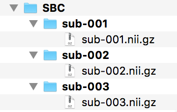
SBC.zip consists of preprocessed fMRI files in standard MNI space for three subjects who participated in a resting state fMRI experiment. Each fMRI file is a 4D file consisting of 70 volumes. You should download the data and unzip it:

unzip SBC.zip

The data should look like this:

Under SBC, make a new directory called seed. You will need the seed directory to hold the Posterior Cingulate Gyrus mask you will create next.

Create Mask of Seed Region

The seed region will be the Posterior Cingulate Gyrus. You will identify the seed region using the Harvard-Oxford Cortical Atlas.

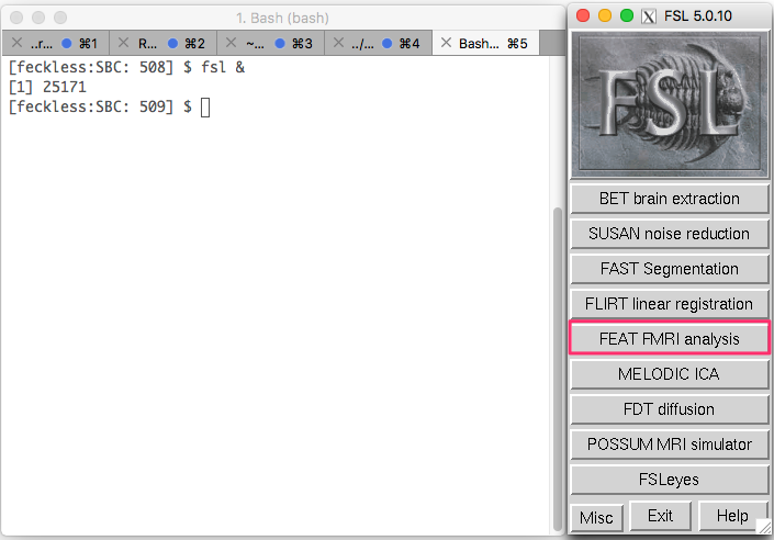
To start FSL, type the following in the terminal:

fsl &

N.B. The & symbol allows you to type commands in this same terminal, instead of having to open a second terminal.

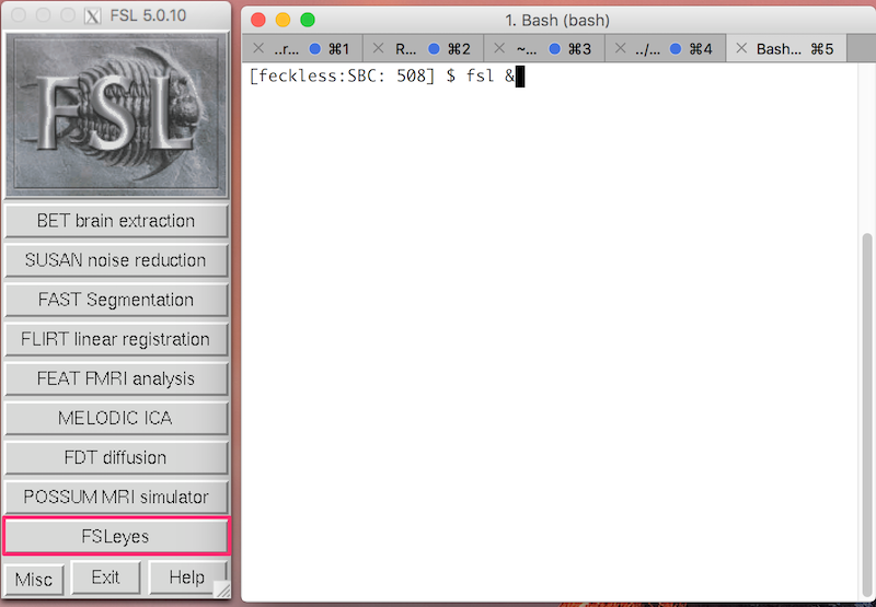
• Click FSLeyes to open the viewer.
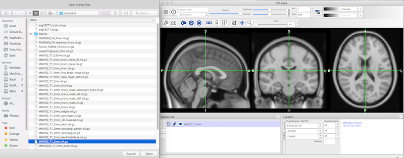
• Click File ➜ Add standard ➜ Select MNI152_T1_2mm_brain.nii.gz ➜ Click Open.
• You will see the standard brain image in three different orientations.

• Click Settings ➜ Ortho View 1 ➜ Atlas panel
• An atlas panel opens on the bottom right.
• Select Atlas search (red box, lower middle).
• Insure Harvard-Oxford Cortical Structural Atlas is selected (purple highlighting).
• Type cing in the search box and check the Cingulate Gyrus, posterior division (lower right) so that it is overlaid on the standard brain.

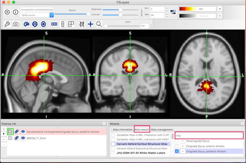
• To save the seed image, click the save symbol (green box, bottom left) next to the seed image.
• Save the image as PCC in the seed directory. If you go to the seed directory, you will see PCC.nii.gz in the folder.
• Leave FSLeyes open.

In the terminal, cd to the seed directory. You are going to binarize the seed image so we can use it as a mask:

fslmaths PCC -thr 0.1 -bin PCC_bin

• In FSLeyes click File ➜ Add from file to compare PCC.nii.gz (before binarization) and PCC_bin.nii.gz (after binarization).
• You can close FSLeyes now.

Extract Time Series from Seed Region

For each subject, you want to extract the average time series from the region defined by the PCC mask. To calculate this value for sub-001, type:

fslmeants -i sub-001 -o sub-001_PCC.txt -m ../seed/PCC_bin

Repeat for sub-002 and sub-003.

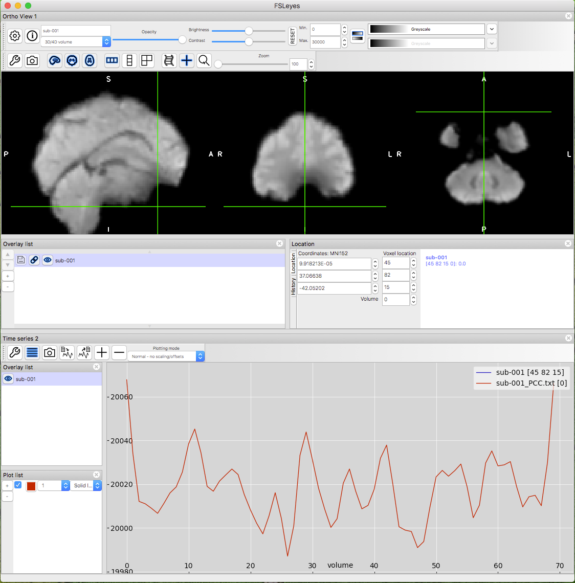
You can view the timecourse in the text file using FSLeyes:

• Display sub-001.nii.gz in FSLeyes (File → Add from file → sub-001.nii.gz)
• On the FSLeyes menu, click View → Time series. You see the time series of the voxel at the crosshairs.
• Move the crosshairs off the brain, so the time series is a zero-line.
• Click Settings → Time series 2 → Import and select the sub-001_PCC.txt file you just created.
• Click OK. You should see the timecourse of the txt file. You can add text files for sub-002 and sub-003 if you wish.
• You can close FSLeyes when you are done.

Run the FSL FEAT First-level Analysis

For each subject, you want to run a first level FEAT analysis showing us the brain regions that have activity correlated to the mean PCC activity.

Start FSL again:

fsl &

Select FEAT FMRI analysis.

• This is FEAT, the FMRI Expert Analysis Tool.
• On the default Data tab, Number of inputs is 1.

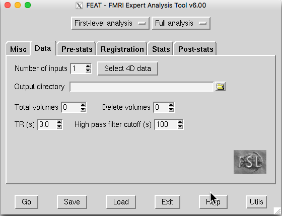
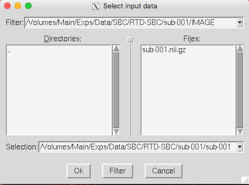
• Click Select 4D data, and a Select input data window will appear.
• Click the yellow folder on the right-hand side and select sub-001.nii.gz.

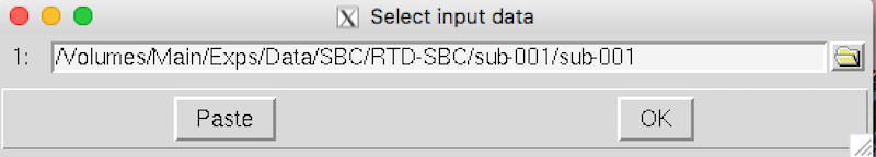
Click OK to close each Select input data window.

If you see the following message, click OK.

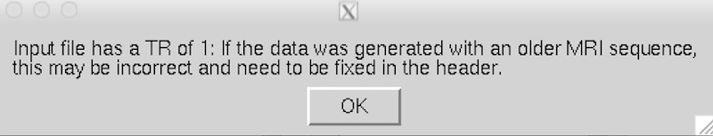
You are back to FEAT – FMRI Expert Analysis Tool* window.

• Click the yellow folder to the right of the Output directory text box.
• A window called Name the output directory will appear.
• Go to the sub-001 folder and click OK.
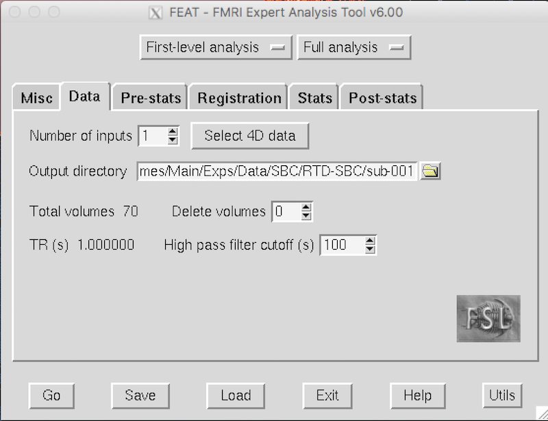
• You have told FSL to create a feat directory called sub-001.feat at the same level as the subject and seed directories.
• The Data tab should look like this:

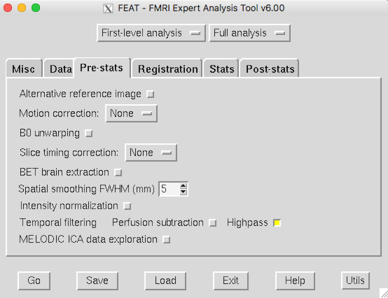
Click the Pre-stats tab. Because this dataset was already preprocessed, you don’t need most of these options. Change the parameters to match the picture:

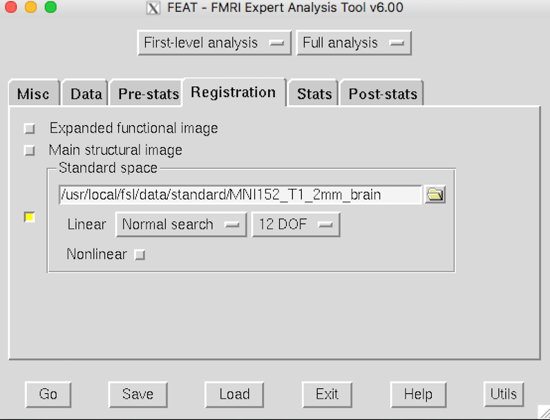
Click the Registration tab and make sure it matches this picture:

Click the Stats tab and then Full model setup:

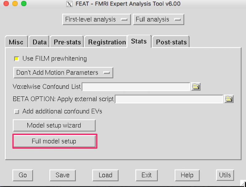
A General Linear Model window will appear.

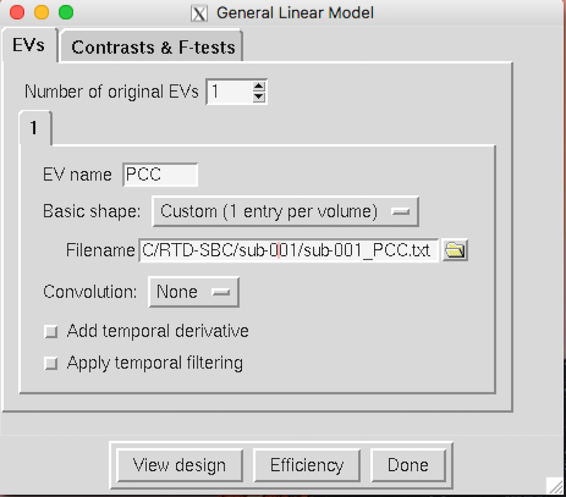
• The Number of original EVs is 1.
• Type PCC for the EV name.
• Select Custom (1 entry per volume) for the Basic shape.
• To the right of the Filename text box, click the yellow folder and select sub-001_PCC.txt This is the mean time series of the PCC for sub-001 and is the statistical regressor in our GLM model.
• The first-level analysis will identify brain voxels that show a significant correlation with the seed (PCC) time series data.
• Select None for Convolution, and deactivate Add temporal derivate and Apply temporal filtering
• Your general linear model should look like this:

• In the same General Linear Model window, click the Contrast & F-tests tab.
• Type PCC in the Title, and click Done.
• A blue and red design matrix is displayed. You can close it.
• You don’t need to change anything in the Post-stats tab.
• You are ready to run the first-level analysis. Click Go now.
• A FEAT Report window will appear in your web browser. You will see Still running. Wait 5-10 minutes for the analysis to finish.
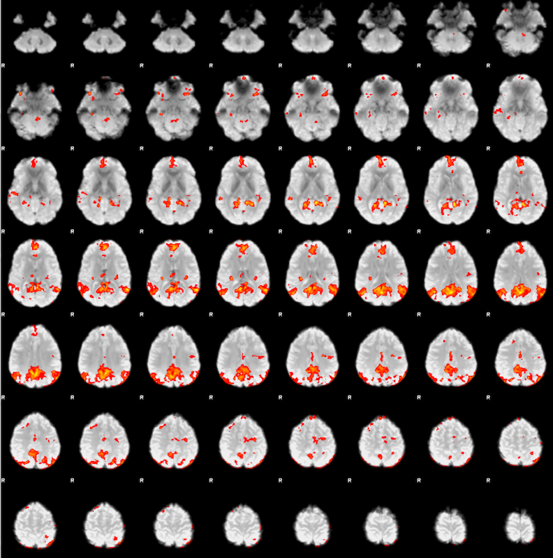
• After the analysis finishes, you see a FEAT Report in the browser. Click Post-stats, and you should be able to see the following results:

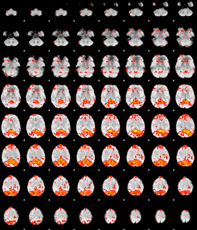
• Click the figure to see the cluster list and the local maxima data.
• You have finished the first-level analysis for sub-001. You can save your model by clicking Save.
• To run a group analysis, you need at least three datasets. You must repeat the above steps for sub-002 and sub-003. There are three values you need to modify:

1. The input file on the *Data* tab: For example, click Select 4D data, and change the input data from sub-001/sub-001.nii.gz to sub-002/sub-002.nii.gz
2. The output directory on the *Data* tab: For example, change the output directory from sub-001 to sub-002.
3. The PCC txt file on the *Stats* tab → Full model setup: For example, change the filename from sub-001/sub-001_PCC.txt sub-002/sub-002_PCC.txt.

• Once you finish the first-level analysis for sub-002, you can expect to see the following results:

Repeat the same steps for sub-003.

The FSL FEAT Higher-level Analysis

In the FEAT – FMRI Expert Analysis Tool Window, select High-level analysis (instead of First-level analysis). The higher level analysis relies on:

1. Each of the individual subject feat analyses AND
2. A description of the GLM model.

Select Each Individual Subject FEAT Analysis

On the Data tab:

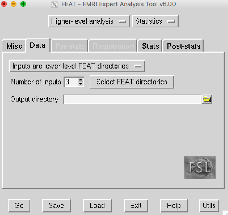
• Select the default option, Inputs are lower-level FEAT directories.
• Number of inputs is 3.
• Click the Select FEAT directories. A Select input data window will appear:

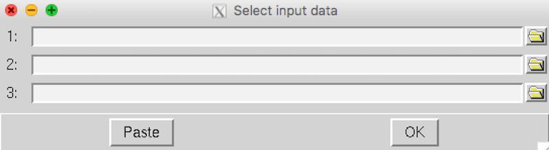
• Click the yellow folder on the right to select the FEAT folder that you had generated from each first-level analysis.
• After selecting the three Feat directories, it will look like this:

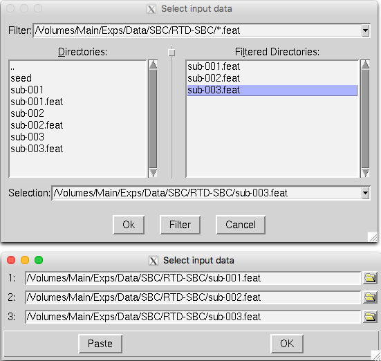
Click OK.

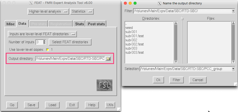
Name an Output Directory

• Click the yellow folder to the right of the Output directory text box, and provide a name for the output directory, e.g. PCC_group (N.B., Don’t put PCC_group inside a subject directory, or you’ll have a hard time finding it later).
• Click OK.

On the Stats tab, click Full model setup. In the General Linear Model window, name the model PCC and insure the interface looks like this:

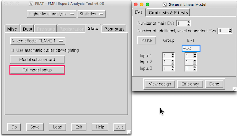
• Click Done to close the General Linear Model window.
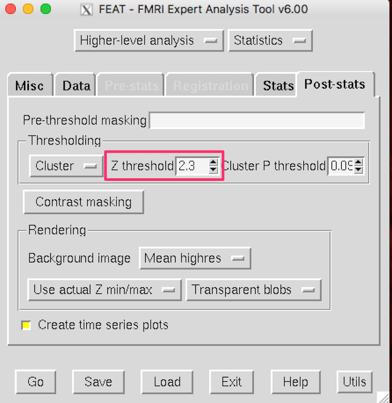
• Because there are so few subjects here, and you want to see some results, you are going to set z down to 2.3 instead of 3.1 on the FEAT Post-stats tab:

Run the Higher-level Analysis

• Click Go to run the Higher-level analysis.
• While you see Still running, you will need to wait a few minutes for the analysis to be done.
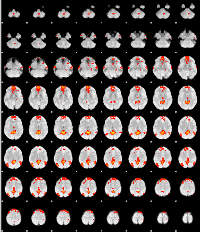
• After 5-10 mins, click Results.
• Then click Results for lower-level contrast 1 (PCC) if it is available, that means it is done. * Click Post-stats, and you should see this:

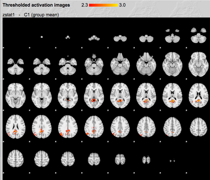
As you can imagine, due to the small sample size (N=3), many voxels do not pass the multiple comparisons correction. You would see a more complete default mode network with more subjects.